Flexible Transducer Arrays
A flexible array conforms to the body. The moment it bends, delay-and-sum no longer knows where its elements are.
Four numbers describe the array
The probe surface is approximated by a cubic. Bend it and watch the 32 elements follow.
Peak deformation 2.20 mm within the 2.5 mm range simulated
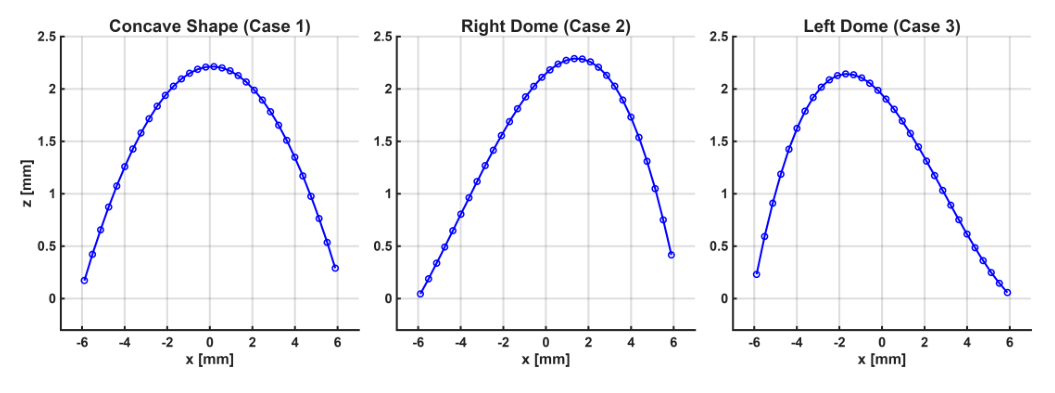
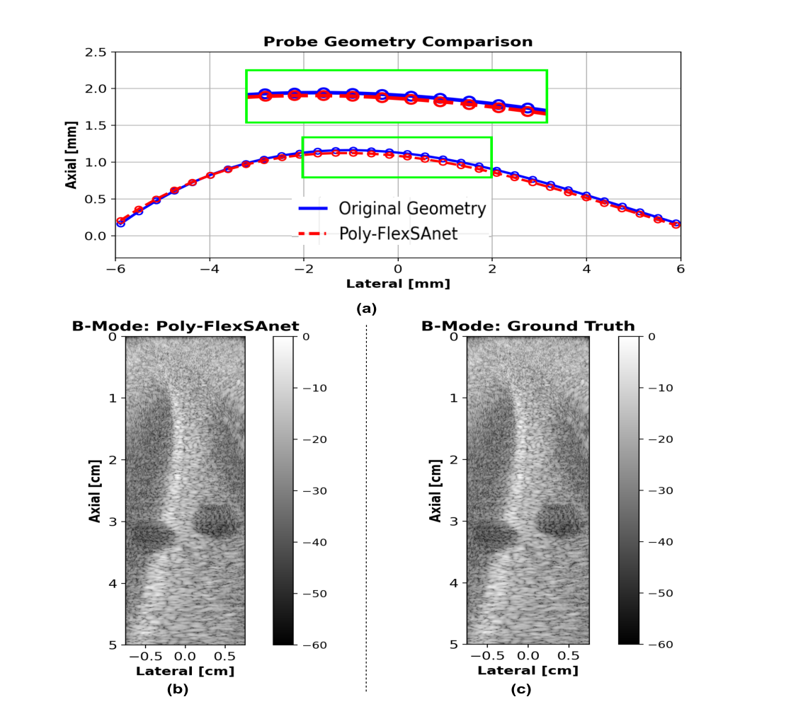
Illustration of the parameterisation described in the paper, not measured data. The paper’s own simulated geometries are in Fig. 1 below.
Bending breaks the beamformer
Ultrasound is often the only modality practical for monitoring an organ continuously. Rigid arrays cannot do it: fixed geometry gives poor contact on a curved surface, and poor contact gives a poor image.
A flexible array solves the contact problem and creates a new one. Delay-and-sum needs element positions to compute time-of-flight delays. When the array conforms, those positions move, and nothing downstream knows where they went. Recovering the geometry is a precondition for reconstructing the image at all.
What has been tried, and what it costs
- External position sensingOptical shape-sensing fibre or MRI guidance. Expensive and complex for continuous monitoring.
- Entropy optimisationSensitive to how the geometry estimate is initialised.
- Spatial coherence & focus metricsOptimised SLSC and iterative gradient energy. Both limited by computational overhead.
- Phase coherenceDegraded by noise and motion artefacts.
- Deep learningPredicts curvature radius only, not the randomness in the geometry. Scarce flexible-array data limits it to one probe and transmit type.
A cubic, and the four coefficients that fix it
Four numbers, regressed directly from raw channel data
Varying the coefficients produces the three deformation types used to build the dataset: concave, right dome and left dome, each a distinct curvature profile of the 32-element array with vertical deformation up to 2.5 mm. Earlier networks predict a single curvature radius, which cannot represent an array that bends unevenly. A cubic can.
- Elements
- 32
- Centre freq.
- 7.5 MHz
- Sampling
- 30 MHz
- Pitch
- 0.38 mm
- Element W × H
- 0.36 × 1 mm
Simulating what a bent array sees
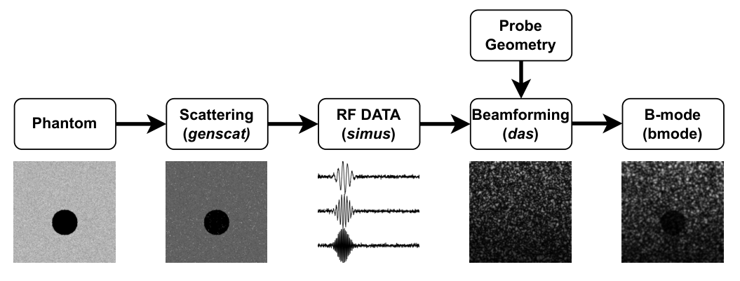
Phantoms are cysts, circular with radii from 0.30 to 0.40 cm, or vessels, horizontal tubes with half-widths from 0.40 to 0.50 cm and half-heights from 0.10 to 0.25 cm. MUST computes transmit delays with txdelay, generates RF channel data with simus, beamforms with DAS and log-compresses with bmode.
One plane wave in
A single plane-wave acquisition gives 32 channels by 2120 temporal samples, covering 5 cm of depth. Using one transmit rather than a synthetic aperture sequence is what keeps the frame rate high.
Two features out
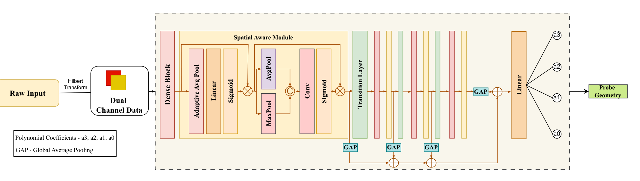
Each channel is converted to its analytic signal by Hilbert transform, then split into envelope and instantaneous phase. The phase channel is what makes the network sensitive to the sub-sample time-of-flight shifts that deformation causes.
Poly-FlexSANet
- Backbone
- Four DenseNet-style blocks, growth rate 16, configuration (6, 12, 24, 16). Transition layers use 1×1 convolution and 2×2 average pooling.
- Attention
- A CBAM-like module after each block. Channel attention weights envelope against phase; spatial attention finds the regions along the time axis that deformation actually touches.
- Multi-scale head
- Global average pooling taps every Spatial-Aware Module rather than only the last, so shallow and deep features both reach the regressor. This and the dual-channel input are the two changes from the FlexSANet baseline.
- Phantoms
- 1800
- Split
- 90 / 10
- Epochs
- 100
- GPU
- RTX 4070
- Optimiser
- Adam, 10−4
- Batch
- 5
Geometry error halves
| Model | RMSE (mm) ↓ | SSIM ↑ |
|---|---|---|
| FlexSANet baseline | 3.09×10⁻³ ± 2.87×10⁻³ | 0.65 ± 0.19 |
| Poly-FlexSANet | 1.55×10⁻³ ± 2.14×10⁻³ | 0.67 ± 0.22 |
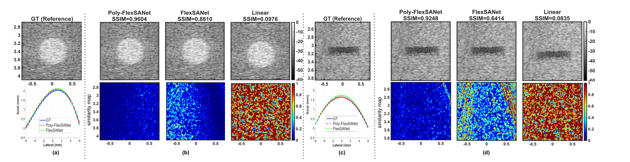
In the similarity maps, blue marks agreement between predicted and ground-truth B-mode images. Across all three deformation types the predicted geometries track the true probe shapes, which is the claim that matters: the model captures diverse curvature, not just a radius.
From simulation to a worn array
Everything here is simulated, and that is the limit to be honest about. The next step is domain adaptation: carrying a network trained on synthetic data across to acquisitions from a physical flexible array. That is the step that turns this into a wearable imaging system rather than a result.
All data in this work is simulation data. No human or preclinical data was used.