Underwater 3-D Acoustical Imaging
Conventional 3-D underwater imaging demands uniform planar arrays with thousands of hydrophones and computationally intensive beamforming. This project replaces the full planar array with orthogonal linear arrays containing as few as 47 elements, achieving real-time volumetric imaging for autonomous underwater vehicle navigation and deep-sea obstacle avoidance.
Why 3-D Sonar Imaging Is Hard
Reconstructing 3-D volumetric images of underwater targets requires a 2-D receiving array and computationally intensive beamforming. The cost scales with the square of the number of sensor elements.
Orthogonal Linear Array Beamforming
An L-shaped arrangement of two perpendicular linear arrays replaces the full 2-D planar aperture. For a 24 × 24 UPA, element count drops from 576 to 47 hydrophones (92% reduction). Product beamforming combines the two beams, reconstructing the 3-D image in parallel across four quadrants.
- Array Type L-shaped at edges of UPA (ELSA)
- Elements 47 hydrophones (vs. 576 for full UPA)
- MLW Improvement 2° narrower main lobe than DAS with UPA
- Ambiguity Asymmetric PSF resolves multi-target ambiguity
- Computation 97× fewer operations than conventional DAS
- Frequency 500 kHz center, 200 kHz wideband operation
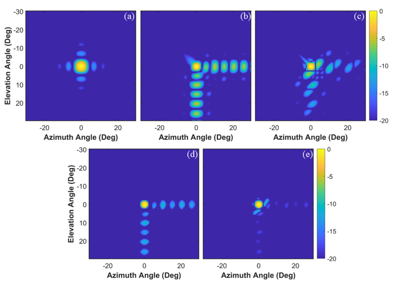
| Array Geometry | Elements | Method | Azimuth MLW | Elevation MLW | PSLL (dB) |
|---|---|---|---|---|---|
| UPA | 576 | DAS | 4° | 4° | −13 |
| ELSA | 47 | DAS | 4° | 4° | −5 |
| ELSA | 47 | Product | 2° | 2° | −7 |
| CSA | 47 | Product | 5° | 5° | −6 |
| CLSA | 47 | Product | 2° | 2° | −7 |
| DCSA | 95 | Product | 2° | 2° | −7 |
From Cross-Correlation to Nonlinear Product Beamforming
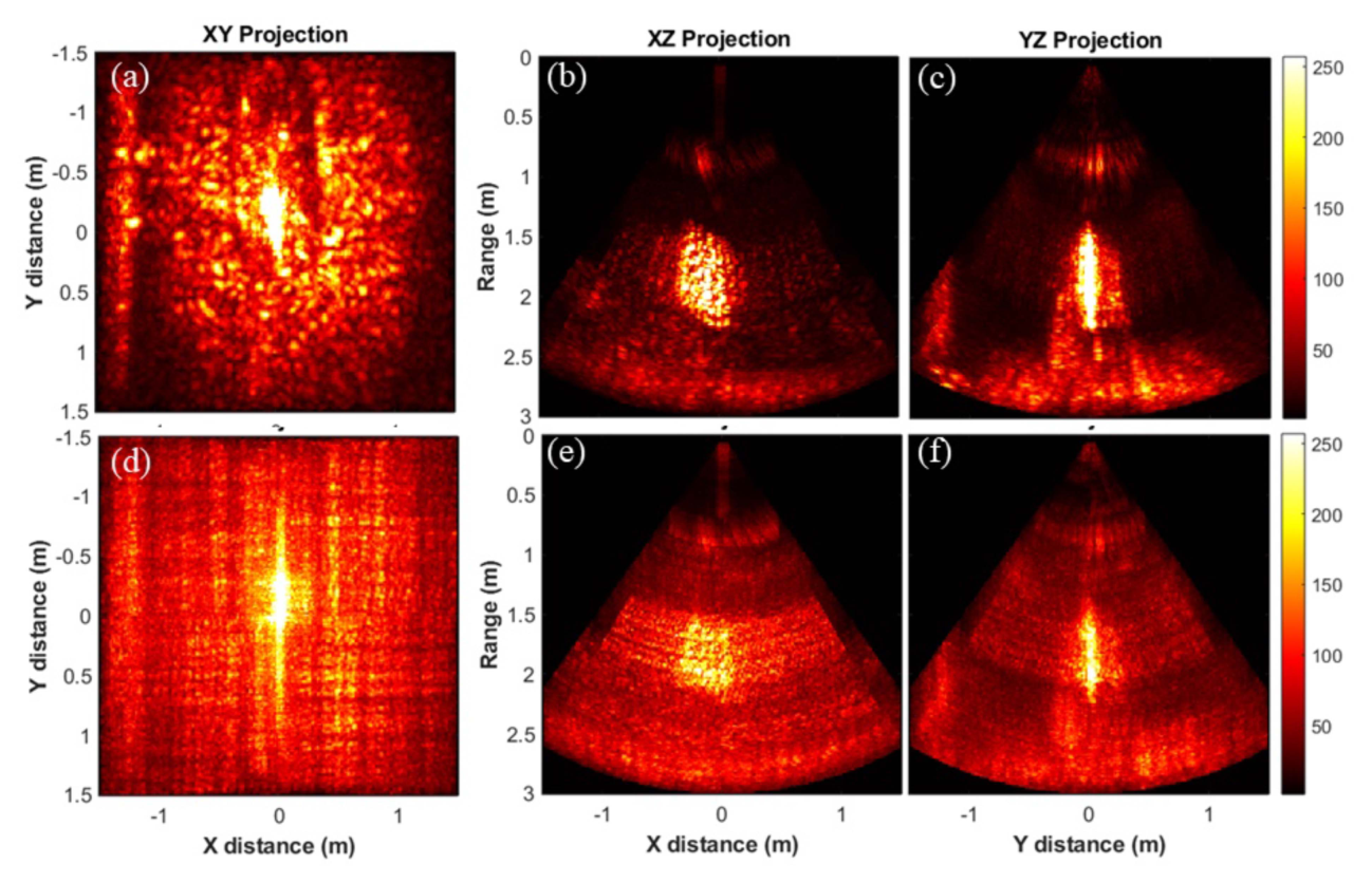
Cross-array spatial cross-correlation multiplies delay-compensated signals of horizontal and vertical arms for directional 3-D beams. The more advanced nonlinear product beamforming on the ELSA uses quadrant-based reconstruction, processing all four quadrants in parallel.
- Cross-Array 22× faster than DAS for 120 × 120 beams (0.39 s vs 8.89 s)
- Product BF 97× fewer operations, single-slice time 0.21 s vs 0.12 s (DAS), but with improved MLW
- DMAS Compared against DMAS: 4 dB PSLL reduction, with 4.8× fewer operations
- Platform Benchmarked on 11th Gen Intel Core i7-1165G7, 2.80 GHz, 8 GB RAM
Compressive Sensing for Wideband Sparse Array Synthesis
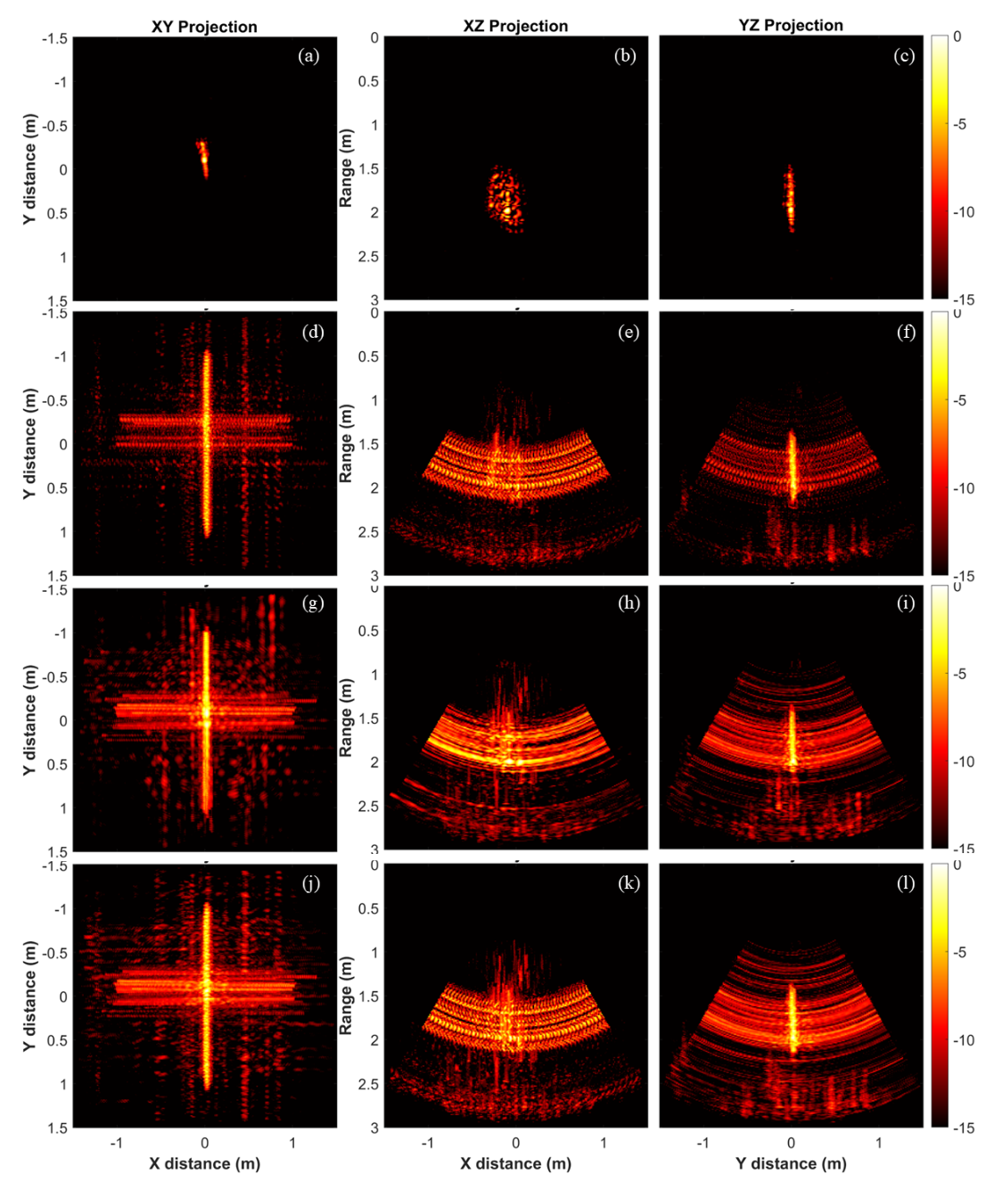
A multitask Bayesian compressive sensing (MTBCS) algorithm jointly optimizes sensor locations across all frequency bins. For ultra-wideband signals (150 to 450 kHz), MTBCS reduced a 10,000-element reference array to 917 elements while maintaining minimum mean-square error.
- Algorithm Multitask Bayesian Compressive Sensing (MTBCS)
- Signal Type Wideband (up to 100% relative bandwidth) and ultra-wideband
- Patterns Frequency-dependent and frequency-invariant beam patterns
- Steering Verified beam steering to (30°, 30°) with sparse array
- Experiments Validated with 96-element uniform array data from NPOL, reduced to 29 elements
Underwater Target Modeling with k-Wave
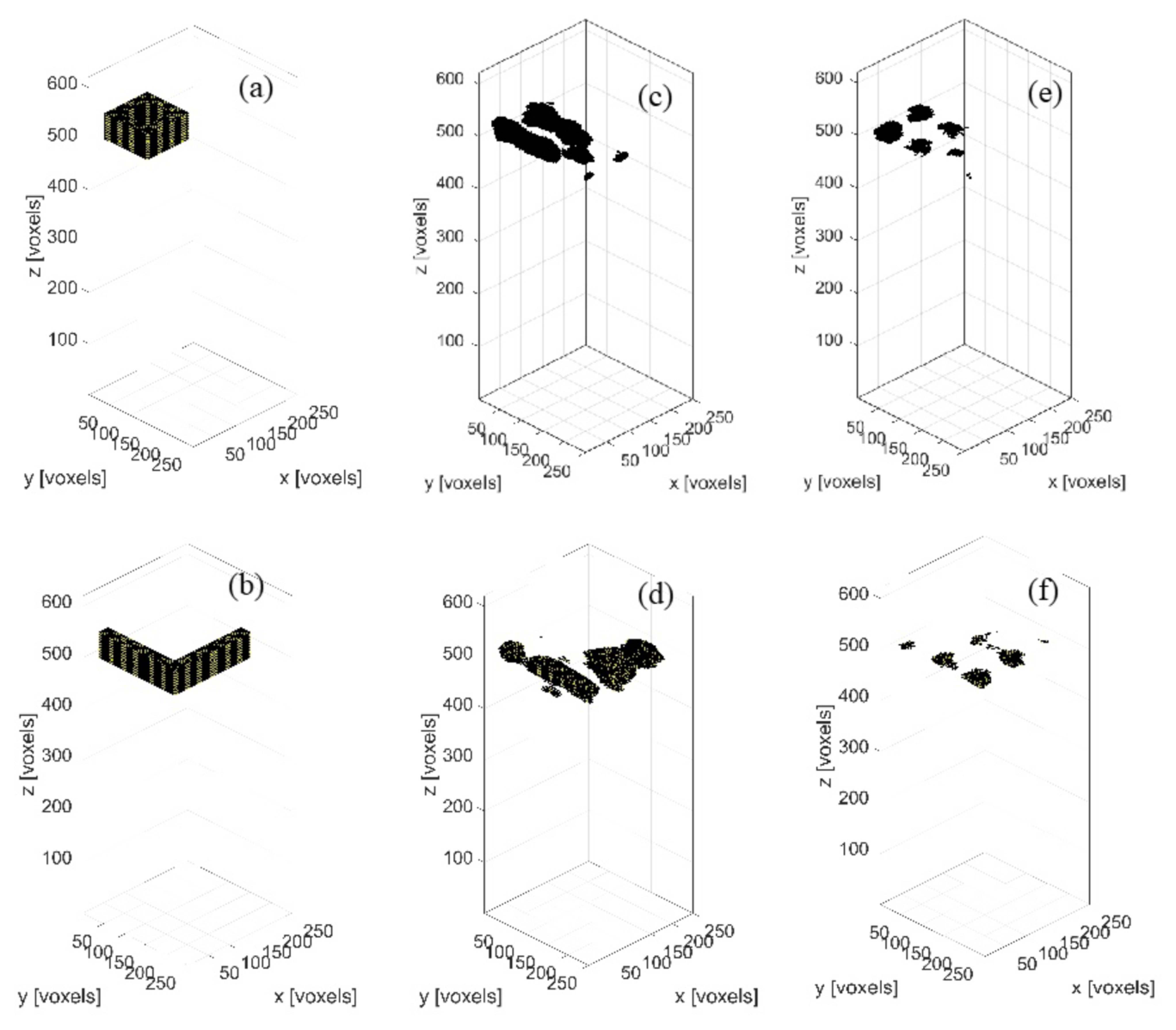
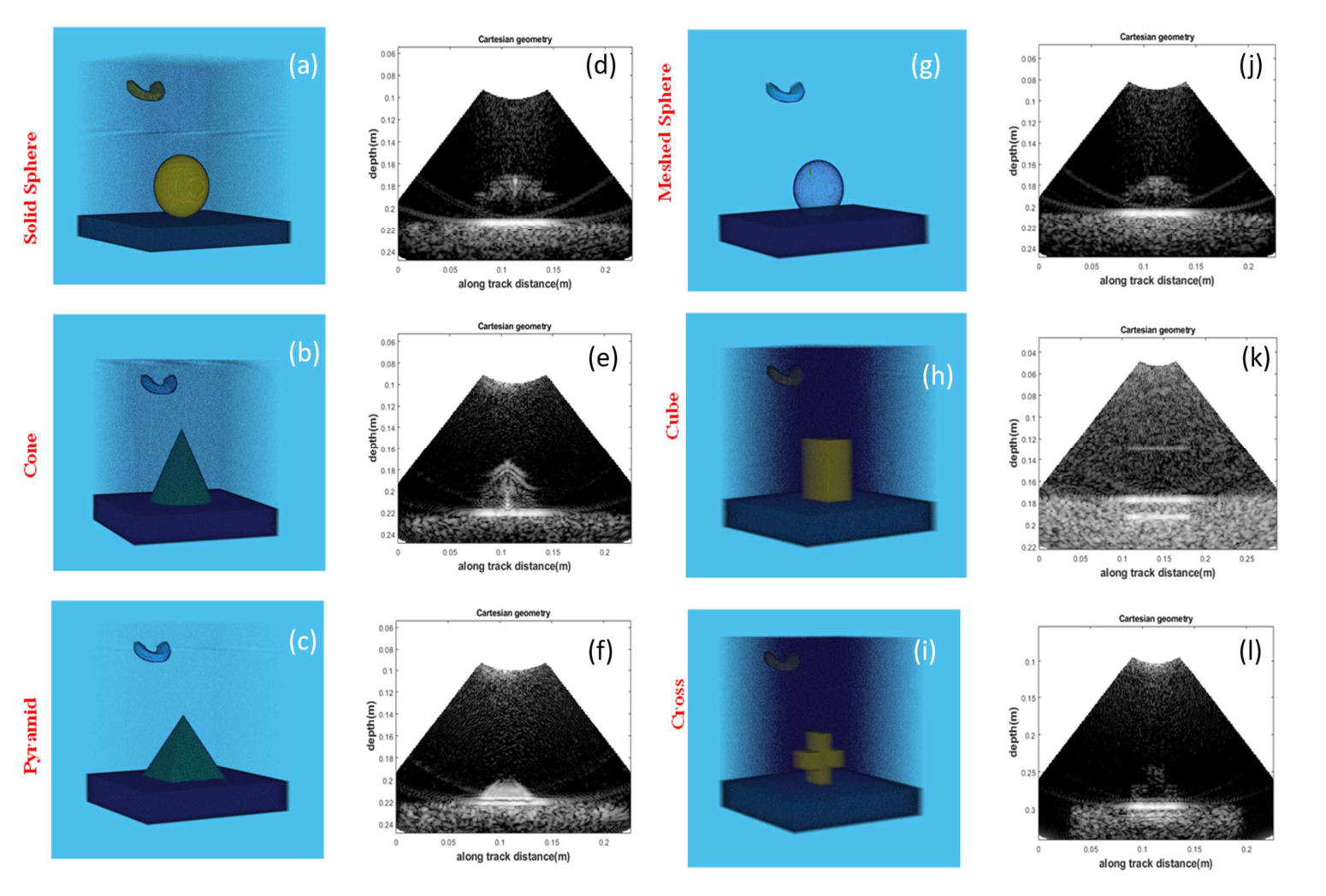
The k-Wave acoustic toolbox solves the wave equation directly, capturing attenuation, reverberation, and speckle that analytical models miss. Two scaling approaches handle deep-water memory constraints while preserving angular resolution. Validated against experimental data from NPOL, Kochi, using a 96-element linear array at 725 kHz.
- Toolbox k-Wave (open-source, MATLAB), time-domain wave equation solver
- Shallow Water 0.4 m × 0.3 m × 0.3 m grid, 1 mm grid points, 725 kHz
- Deep Water Scaled-down approach: factor 1/2.5 for practical memory usage
- Targets Sphere, cube, cone, pyramid, meshed sphere, cross-shaped structures
- Materials Mild steel: 3000 m/s acoustic speed, 7850 kg/m³ density
- Validation Simulated vs experimental images at NPOL show matching target shapes
| Method | Operations | Time (s) | Speedup |
|---|---|---|---|
| DAS (UPA) | 6,221,952 | 0.1210 | 1× |
| CZT | 3.57 × 10¹¹ | 1.0630 | 0.11× |
| DM (Frequency) | 1.99 × 10¹° | 96.2032 | 0.001× |
| Proposed (ELSA) | 864,000 | 0.0052 | 23× |
Published Work
Six peer-reviewed publications spanning array design, beamforming algorithms, sparse synthesis, and simulation validation.