Ultrasound Front End
Everything that decides image quality happens between the transducer and the first displayed pixel. That stretch of the system has a fixed power budget and no time to think.
The receive chain is where the image is won or lost
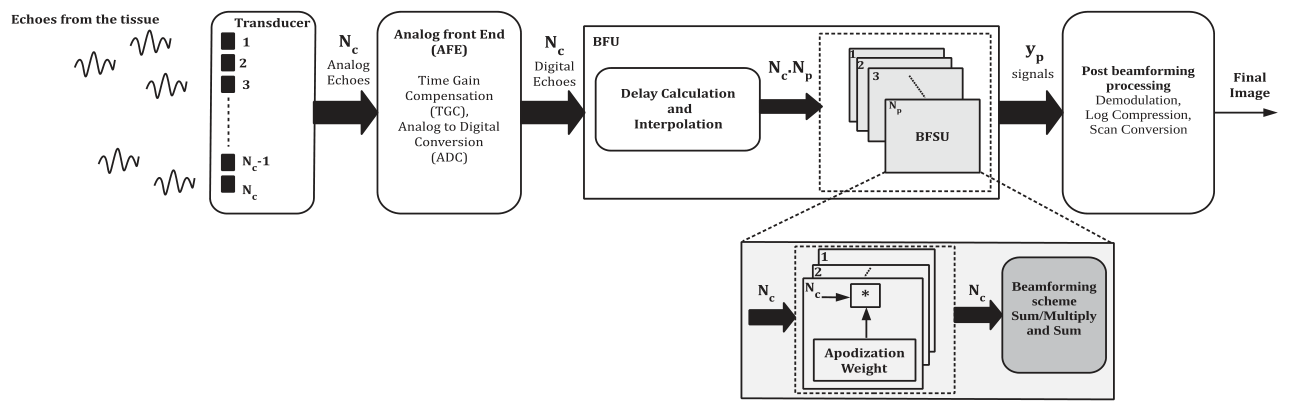
Echoes arriving at a transducer array are weak, wideband and arrive at different times at every element. The analog front end compensates gain with depth and digitises them; the beamforming unit then delays, weights and sums them into one line of the image. Whatever information that chain discards is gone before any image processing runs.
Almost every commercial system uses delay and sum beamforming, because it is cheap. It also assumes the medium is a homogeneous diffuse scatterer, so delays and apodization weights depend only on the Euclidean distance from a pixel to each element. That assumption holds for speckle and fails for bone, needles and vessel walls, whose reflections are highly directive.
Better beamformers exist. Delay multiply and sum recovers resolution and contrast, but it generates harmonics that must stay inside the processable band of the system, which restricts it to lower transducer frequencies. Minimum variance methods compute weights from the data itself, at a cost of O(n3) in the aperture size: roughly 98.78 GOPs per frame for a 368 by 128 frame. Deep beamformers reconstruct beautifully and do not fit on an edge device.
The work below treats that as a hardware question rather than an algorithm question. Each project asks what the receive chain can be made to do inside the resource and latency budget of an FPGA or an embedded GPU.
Let each pixel choose its own beamformer
A system that ships one beamforming scheme has to pick the compromise in advance. Delay and sum suffers high sidelobes and limited resolution; delay multiply and sum gives finer detail at depth but cannot be used above the frequency at which its harmonics leave the processable band. Choosing between them is a property of the transducer and of the tissue region, not of the product.
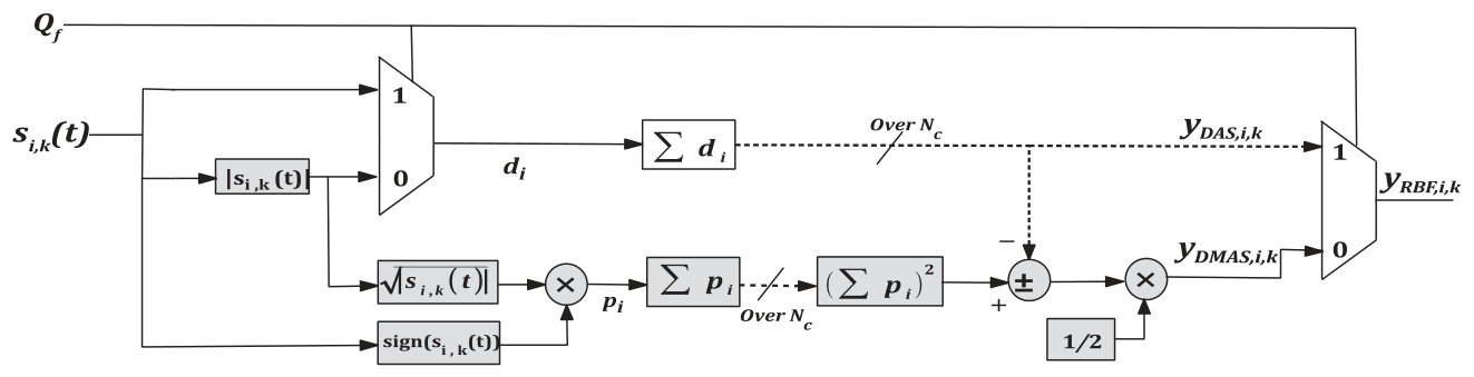
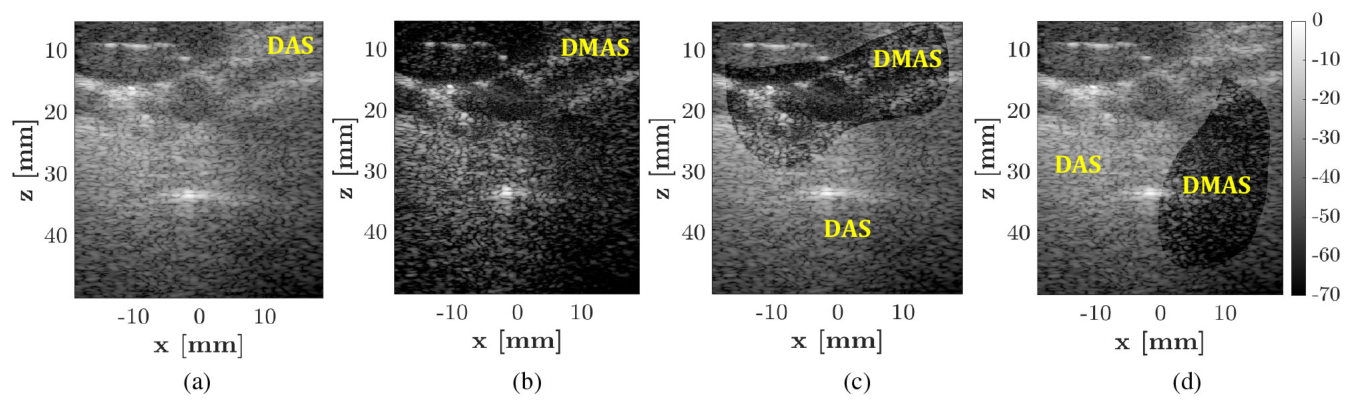
Two architectures make that choice reconfigurable with almost no extra logic. Both modify the existing delay and sum and delay multiply and sum datapaths so a single core can run either, selected by a flag Qf derived from the transducer centre frequency. Because each core is built per pixel and pixels are independent, the selection can also be made per pixel: regions that need resolution get delay multiply and sum, regions that need contrast to noise ratio get delay and sum.
The two architectures
- FBRA
- Fully bypassed reconfigurable architecture. The multiply stage is bypassed rather than duplicated, so it occupies less logic than the alternative. Preferable where hardware savings are the priority.
- MEBRA
- Multiplier embedded reconfigurable architecture. Slightly larger, with the cumulative sum transferred from source to destination through the same datapath in both modes.
| Architecture | Logic LUTs | Registers | DSPs |
|---|---|---|---|
| FBRA | 222 of 17600 | 196 of 35200 | 1 of 80 |
| MEBRA | 251 of 17600 | 222 of 35200 | 1 of 80 |
- Device
- xc7z010clg400-1
- Clock
- 125 MHz
- Channels
- 64 / 128 / 256
- Square root latency
- 5 clocks
- Resolution
- 0.33 mm
Hardware increment is close to negligible across Nc = 64, 128 and 256, so the complexity of the reconfigurable core is not constrained by aperture size. Clock counts scale with Nc as expected, with TDAS = Nc + 1. The imaging datasets were sampled at 20.832 MHz from a 5.2 MHz transducer.
Pixel level reconfigurability was demonstrated in simulation on an in vivo carotid artery dataset, with different regions of the same frame beamformed by different schemes.
Weights that follow the reflector, not the geometry
Apodization weights the signals across the receive aperture to suppress sidelobes. Under the diffuse assumption those weights are a function of pixel position alone, and the window sits centred on the pixel. A specular reflector, a bone surface or a needle in a guided intervention, sends its energy in a direction set by the angle of incidence and the reflector orientation. The aperture that actually receives that energy is not the one centred on the pixel, so the structure appears distorted or vanishes altogether.
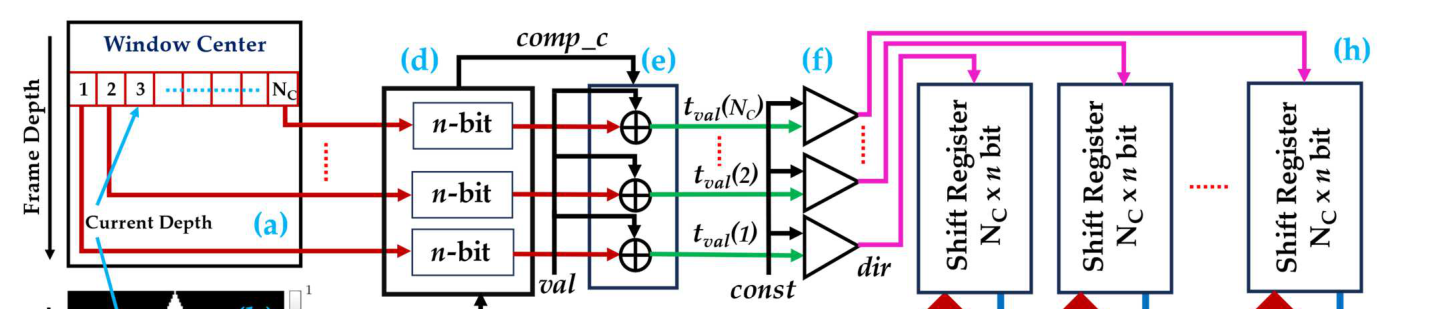
Data adaptive beamforming solves this by computing weights from received data, and pays for it in covariance estimation. Raster apodization design takes a different route: it adjusts the apodization coefficients at pixel level in hardware according to reflection directivity, estimating coefficients for every pixel at a fixed depth simultaneously, in the manner of a raster scan, while reusing a single reference apodization window.
- Device
- XCZ7010clg400-1
- Clock
- 125 MHz
- Row latency
- 260 clocks
- Transmit
- 7.6 MHz, one plane wave
- Steering
- 18°
All raster apodization design block units for a row execute in parallel, giving a latency of 260 clock cycles for a single row. Validation used a Verasonics Vantage 128 with an L11-5v 128 element linear array, imaging a custom needle guided at 20° into the tissue mimicking region of a CIRS Model 769 flow phantom, at a speed of sound of 1540 m/s and attenuation of 0.7 dB/cm/MHz. Coefficients produced by the FPGA were checked against the same computation in MATLAB, and beamformed images were compared against conventional apodization at a 60 dB dynamic range.
A capsule network small enough to synthesise
Adaptive and deep beamformers improve images and do not fit on the devices that would benefit most. CapsBeam is a capsule network beamformer that operates directly on raw radio frequency data and returns the envelope of the beamformed data, from a single non steered plane wave insonification. It was then made deployable, rather than being reported as a model and left there.
Against standard delay and sum, in vitro data showed a 32.31% increase in contrast with gains of 16.54% axial and 6.7% lateral resolution; in silico data showed 26% contrast with 13.6% axial and 21.5% lateral. In vivo, artefacts were reduced. Getting from there onto a board took three separate reductions: multi layer LookAhead Kernel Pruning compressed the model by 85% without affecting image quality, quantisation from 32 bit to 16 bit doubled the data moved per transaction, and the exponential in the routing algorithm was replaced by a Taylor expansion of multiplications and additions.

| Model | Frames per second |
|---|---|
| CapsBeam optimised | 2.07 |
| Tiny-VBF | 1.48 |
| Tiny-CNN | 1.41 |
| CNN | 0.015 |
The accelerator reaches 30 GOPS on the convolution operation and 17.4 GOPS on dynamic routing. Compared against minimum variance beamforming at 98.78 GOPs per frame, the optimised model needs roughly 6.
Consecutive frames are nearly the same frame
A tissue adaptive network run at high frame rate recomputes, for every frame, feature maps that barely changed since the last one. FeatuReBeam exploits that similarity to skip redundant computation, and borrows the (m,k) model from real time scheduling to keep the skipping honest: at least m out of every k consecutive frames are computed in full, which bounds how far output quality can drift before a mandatory frame resets it.
Each frame is classified as mandatory or optional. Mandatory frames run the pretrained beamformer end to end and publish their feature maps; optional frames reuse the similar maps and compute only what differs. Inter frame similarity determines the window size k and the filter choosing rate per layer.

Evaluation used U-Net and GoogLeNet based beamformers on in vitro and in vivo data. The method cut computational complexity by more than half while preserving the image quality of the original models, and outperformed both magnitude based and feature map based filter pruning on computational reduction and on output image quality.
The whole chain, in something you can carry
Portable point of care systems have generally chased focused transmit at low frame rate, extending a 16 or 32 channel receive aperture to reach acceptable image quality. High frame rate imaging with non steered plane wave transmit needs a different pipeline. This prototype pairs a programmable handheld acquisition platform, built around two integrated low power 32 channel analog front ends supporting 128 channel transmit and 64 channel receive, with an Nvidia Clara AGX development kit carrying a 24 GB GPU.
Raw radio frequency data is acquired with non steered plane wave transmit, passed through a host system to the Clara AGX, and beamformed there. Six beamformers were implemented in GPU accelerated Python with CuPy: delay and sum on radio frequency and on in phase and quadrature data, pth root delay and sum, baseband delay multiply and sum, and two Fourier domain techniques, Lu’s method and Stolt’s f-k migration.
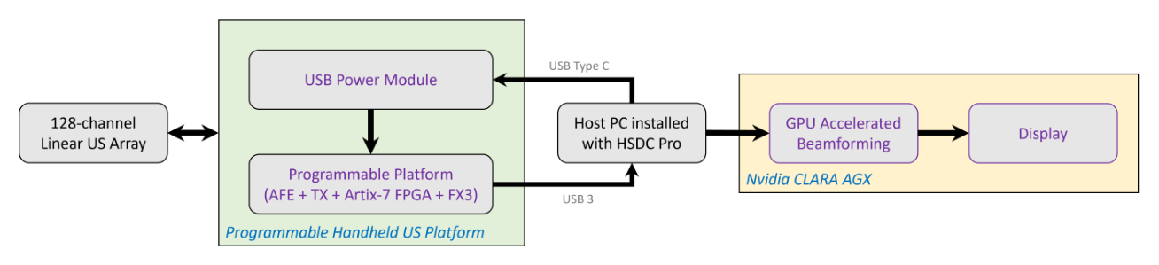
- Transmit / receive
- 128 ch / 64 ch
- Centre freq.
- 7.5 MHz
- Sampling
- 50 MHz
- ADC precision
- 10 bit
- Footprint
- 150 × 100 mm
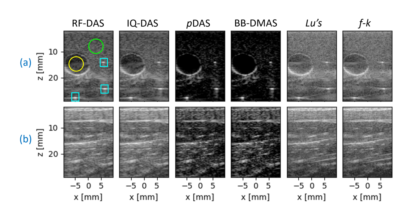
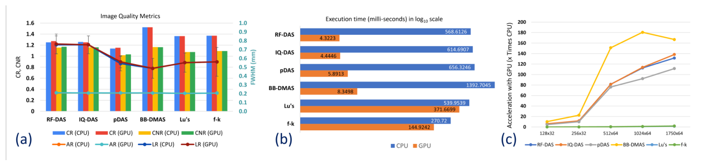
Image quality quantified by standard contrast and resolution metrics was comparable to the CPU implementation. Speedup reached as high as 180 times the CPU implementation for larger imaging grids with RF-DAS, IQ-DAS, pDAS and BB-DMAS, falling to around 5 times for the smallest grids. Lu’s method and f-k migration accelerated least, which the authors flag as needing further work.